Short Answer
Main Explanation
The Sachs–Wolfe effect is a gravitational redshift of cosmic microwave background (CMB) photons caused by variations in the gravitational potential across the sky. It was first described by Rainer K. Sachs and Arthur M. Wolfe in a 1967 paper that integrated the equations for linear perturbations of a Friedmann cosmological model and the lightlike geodesics of the perturbed spacetime. The effect is the predominant source of CMB temperature fluctuations on angular scales larger than about ten degrees, making it a cornerstone of modern cosmology.
To understand the effect, recall that the CMB is relic radiation released when the universe became transparent at recombination, about 380,000 years after the Big Bang. At that time, the universe was not perfectly smooth: regions of slightly higher density had deeper gravitational potential wells. Photons climbing out of a potential well lose energy and are redshifted, while photons falling into a potential hill gain energy and are blueshifted. The Sachs–Wolfe effect translates these potential differences into the large-angle temperature anisotropies we observe.
The effect is usually divided into two parts. The non-integrated Sachs–Wolfe effect (often called the ordinary Sachs–Wolfe effect) occurs at the surface of last scattering. The integrated Sachs–Wolfe effect (ISW) occurs along the photon’s path from the surface of last scattering to Earth, whenever gravitational potentials evolve with time. In a matter-dominated universe, large-scale potential wells and hills remain nearly constant, so the integrated effect is small. But when the universe is dominated by radiation or dark energy, potentials change, and the ISW effect becomes important.
The ordinary Sachs–Wolfe effect produces a temperature shift ΔT = φ/(3c²), where φ is the gravitational potential. This is three times smaller than a naive expectation of φ/c². The factor of three arises because the universe was expanding as the 2/3 power of time at recombination, and a high potential makes clocks—including the expansion clock—run faster, cancelling 2/3 of the naive redshift. The integrated effect gives ΔT = 2Δφ/c², where Δφ is the change in potential while the photon traverses the well. The factor of 2 is the same factor that appears in the deflection of starlight by the Sun.
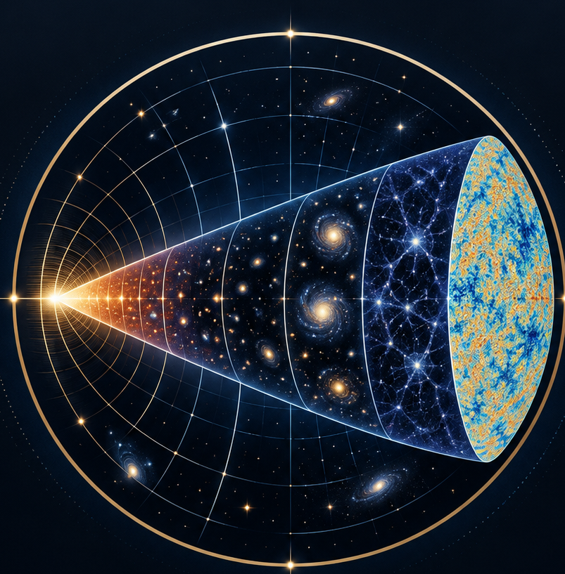
The Sachs–Wolfe effect is intimately connected to the timeline of the universe. The CMB was emitted at recombination, but the potential fluctuations that cause the ordinary effect were seeded by inflation in the first fraction of a second. The late-time integrated effect is sensitive to dark energy, which began dominating the expansion a few billion years ago. Thus, measuring the Sachs–Wolfe effect across different angular scales provides a window into both the very early universe and its recent acceleration.
Cosmic Epochs and the Sachs–Wolfe Effect
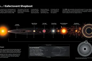
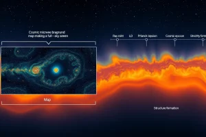
The following table summarizes the major epochs of cosmic history and their connection to the Sachs–Wolfe effect. The ordinary effect is imprinted at recombination, while the integrated effect operates during radiation domination (early ISW) and dark energy domination (late ISW).
| Epoch | Time after Big Bang | Temperature | Redshift | Key Events |
|---|---|---|---|---|
| Planck epoch | <10⁻⁴³ s | >10³² K | — | Quantum gravity; all forces unified |
| Grand Unification epoch | 10⁻⁴³–10⁻³⁶ s | 10³²–10²⁷ K | — | Strong force separates |
| Inflationary epoch | 10⁻³⁶–10⁻³² s | ~10²⁷ K | — | Exponential expansion; seeds density fluctuations |
| Electroweak epoch | 10⁻³²–10⁻¹² s | 10²⁷–10¹⁵ K | — | Weak and electromagnetic forces separate |
| Quark epoch | 10⁻¹²–10⁻⁶ s | 10¹⁵–10¹² K | — | Quarks, leptons, and gluons dominate |
| Hadron epoch | 10⁻⁶–1 s | 10¹²–10¹⁰ K | — | Quarks combine into hadrons |
| Lepton epoch | 1–10 s | 10¹⁰–10⁹ K | — | Leptons and antileptons annihilate |
| Photon epoch | 10 s–380,000 yr | 10⁹–3000 K | 10⁹–1100 | Photons dominate; Big Bang nucleosynthesis |
| Recombination | ~380,000 yr | ~3000 K | ~1100 | First atoms form; CMB released; ordinary SW effect imprinted |
| Dark Ages | 380,000 yr–150 Myr | 3000–60 K | 1100–20 | Neutral hydrogen; no stars |
| Reionization | 150 Myr–1 Gyr | 60–20 K | 20–6 | First stars and galaxies ionize gas |
| Structure Formation | 1 Gyr–present | <20 K | <6 | Galaxies, clusters, large-scale structure; late ISW from dark energy |
Concept
Definition
The Sachs–Wolfe effect is the change in the observed temperature of cosmic microwave background photons caused by gravitational redshift as the photons travel through an inhomogeneous universe. It is a direct consequence of general relativity and the presence of density perturbations.
How It Works
At the surface of last scattering, photons are emitted from regions with slightly different gravitational potentials. A photon emitted from the bottom of a potential well must climb out, losing energy and appearing redshifted (cooler). A photon emitted from a potential hill falls inward, gaining energy and appearing blueshifted (hotter). Because the potential fluctuations are largest on very large scales, the Sachs–Wolfe effect dominates the CMB temperature anisotropy on angular scales greater than about ten degrees.
For the integrated effect, the potential itself changes while the photon is in transit. If a potential well deepens after the photon has entered it, the photon loses more energy climbing out than it gained falling in, producing a net redshift. This happens when the universe’s expansion is dominated by radiation (early ISW) or dark energy (late ISW).
Equation
For the ordinary Sachs–Wolfe effect, the temperature fluctuation is:
ΔT / T = (1/3) Φ / c²
where Φ is the gravitational potential perturbation. For the integrated Sachs–Wolfe effect, the temperature fluctuation is:
ΔT / T = 2 ΔΦ / c²
where ΔΦ is the change in the potential along the photon’s path.
Example
Consider a large overdense region at the surface of last scattering. Its gravitational potential well is deeper than average. A CMB photon emitted from that region loses energy as it climbs out, so it arrives at Earth with a lower temperature than the average CMB. On a map of the CMB, that region appears as a cold spot on angular scales larger than about ten degrees. Conversely, an underdense region appears as a hot spot.
Observable Consequences
- The Sachs–Wolfe effect produces a plateau in the CMB angular power spectrum at low multipoles (large angular scales).
- The late integrated Sachs–Wolfe effect creates a correlation between the CMB and the large-scale distribution of galaxies, because the same potential wells that redshift CMB photons also lens and cluster galaxies.
- Detection of the late ISW effect provides independent evidence for dark energy, since a cosmological constant causes gravitational potentials to decay.
Common Misconceptions
- Misconception: The Sachs–Wolfe effect is a Doppler shift. Reality: It is a gravitational redshift, not a motion-induced Doppler shift.
- Misconception: The ordinary effect should be ΔT = Φ/c². Reality: The expansion of the universe cancels 2/3 of the naive shift, giving ΔT = Φ/(3c²).
- Misconception: The integrated effect only occurs because of dark energy. Reality: An early integrated effect also occurs during the radiation-dominated era, though it is subdominant on the scales probed by the CMB.
Why It Matters
The Sachs–Wolfe effect is one of the cleanest links between the very early universe and what we observe today. The large-angle CMB anisotropies it produces are a direct imprint of the primordial density perturbations generated during inflation. By measuring the amplitude and scale dependence of these anisotropies, cosmologists can test inflationary models and constrain the physics of the Planck epoch.
The integrated Sachs–Wolfe effect is equally important for the late universe. Because dark energy causes gravitational potentials to decay, the late ISW signal is a smoking gun for cosmic acceleration. Cross-correlating CMB maps from Planck with galaxy surveys has detected this signal at high significance, providing independent confirmation of the Lambda-CDM model. The effect also helps break degeneracies between dark energy and modified gravity theories, since different models predict different evolution of gravitational potentials.
Finally, the Sachs–Wolfe effect connects the CMB to the formation of large-scale structure. The same potential wells that redshift CMB photons later grow into galaxy clusters and superclusters. Studying the ISW effect therefore links the earliest observable epoch—recombination—to the present-day cosmic web.
Evidence / Sources
The Sachs–Wolfe effect was first predicted in a 1967 paper by Rainer K. Sachs and Arthur M. Wolfe, who estimated that density fluctuations of order 10% over scales of 1000 Mpc would produce CMB anisotropies of about 1%. The effect remained theoretical until the COBE satellite discovered large-angle CMB anisotropies in 1992. Subsequent missions—WMAP and Planck—measured the angular power spectrum with increasing precision, confirming the predicted Sachs–Wolfe plateau at low multipoles. The late integrated Sachs–Wolfe effect has been detected through cross-correlations between CMB maps and large-scale structure surveys, providing direct evidence for dark energy.
Key sources include the original Sachs & Wolfe (1967) paper, the Wikipedia overview of the effect, and Ned Wright’s cosmology tutorial, which explains the factor of 3 and factor of 2 in accessible terms.
Related Registry Entries
Last reviewed / updated: September 8, 2026
FAQ
What causes the Sachs–Wolfe effect?
Variations in gravitational potential across the universe. CMB photons lose energy climbing out of potential wells and gain energy falling into potential hills, producing temperature anisotropies.
What is the difference between the ordinary and integrated Sachs–Wolfe effects?
The ordinary effect occurs at the surface of last scattering, while the integrated effect accumulates along the photon's path as gravitational potentials evolve. The ordinary effect dominates large angular scales; the integrated effect is important when the universe is radiation- or dark-energy-dominated.
Why is the ordinary Sachs–Wolfe effect three times smaller than a naive estimate?
Because the universe was expanding as the 2/3 power of time at recombination, and a high gravitational potential makes clocks run faster, cancelling 2/3 of the naive gravitational redshift.
How does the Sachs–Wolfe effect provide evidence for dark energy?
The late integrated Sachs–Wolfe effect arises because dark energy causes gravitational potentials to decay. Cross-correlating CMB maps with large-scale structure reveals this late ISW signal, supporting dark energy.
Which missions have measured the Sachs–Wolfe effect?
COBE first detected large-angle CMB anisotropies, WMAP measured the angular power spectrum including the Sachs–Wolfe plateau, and Planck refined these measurements with higher resolution and sensitivity.
Leave a Reply