Short Answer
Main Explanation
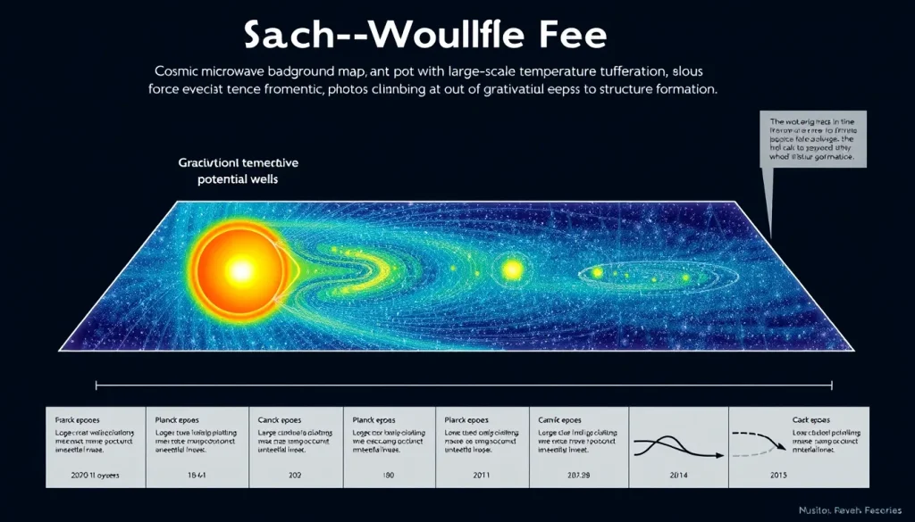
The Sachs–Wolfe effect, named after Rainer K. Sachs and Arthur M. Wolfe, is a fundamental mechanism by which the cosmic microwave background (CMB) acquires temperature anisotropies. It arises from gravitational redshift: photons from the CMB lose energy as they climb out of gravitational potential wells created by density fluctuations in the early universe. This effect is the dominant source of CMB fluctuations on angular scales larger than about ten degrees (source 1). The effect was first predicted in 1967 by Sachs and Wolfe, who integrated the geodesic equation in a perturbed Friedmann–Robertson–Walker metric (source 4). It is a cornerstone of modern cosmology, providing a direct link between the primordial density fluctuations and the observed temperature map of the CMB.
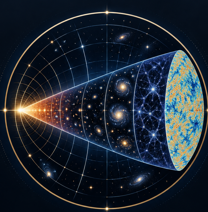
The CMB itself is the relic radiation from the hot, dense early universe, released when photons decoupled from matter at a redshift of about z ≈ 1000 (source 2). At that time, the universe was filled with a nearly uniform plasma, but tiny density fluctuations—seeded by quantum fluctuations during inflation—left imprints on the radiation. The Sachs–Wolfe effect is one of the primary ways these imprints appear.
To understand the effect, consider a photon that originates at the surface of last scattering. If it emerges from a region of higher density, it must climb out of a gravitational potential well, losing energy and appearing cooler. Conversely, a photon from a lower-density region gains energy and appears hotter. This gravitational redshift (or blueshift) creates temperature variations across the sky. Additionally, there is a time-delay effect: photons from overdense regions are scattered later, when the universe is slightly cooler, further contributing to the anisotropy. Both effects together constitute the non-integrated Sachs–Wolfe effect (source 1).
The integrated Sachs–Wolfe (ISW) effect occurs after last scattering, as photons travel through evolving gravitational potentials. If the universe is dominated by matter, the potentials are constant, and no net effect occurs. But if the universe is dominated by radiation or dark energy, the potentials decay, causing a net redshift or blueshift (source 1). The ISW effect is particularly important for studying dark energy, as it imprints additional large-scale anisotropies.
The Sachs–Wolfe effect is not just a theoretical curiosity; it has been measured with high precision by missions such as COBE, WMAP, and Planck. These observations confirm the predictions of the Lambda-CDM model, which describes a universe composed of dark energy, cold dark matter, and ordinary matter, with initial fluctuations generated by inflation.
To place the effect in context, it is helpful to review the major epochs of cosmic history. The table below summarizes the key phases from the Planck epoch to the present day.
| Epoch | Time after Big Bang | Redshift | Temperature | Key Events |
|---|---|---|---|---|
| Planck epoch | < 10-43 s | > 1032 | > 1032 K | Quantum gravity effects dominate; all forces unified |
| Grand Unification epoch | 10-43 to 10-36 s | 1032 to 1028 | 1032 to 1028 K | Strong force separates from electroweak |
| Inflationary epoch | 10-36 to 10-32 s | 1028 to 1022 | 1028 to 1022 K | Exponential expansion; seeds of structure |
| Electroweak epoch | 10-32 to 10-12 s | 1022 to 1015 | 1022 to 1015 K | Electromagnetic and weak forces separate |
| Quark epoch | 10-12 to 10-6 s | 1015 to 1012 | 1015 to 1012 K | Quarks and gluons form quark-gluon plasma |
| Hadron epoch | 10-6 to 1 s | 1012 to 1010 | 1012 to 1010 K | Quarks combine into hadrons; protons and neutrons |
| Lepton epoch | 1 s to 10 s | 1010 to 109 | 1010 to 109 K | Leptons dominate; neutrinos decouple |
| Photon epoch | 10 s to 380,000 yr | 109 to 1100 | 109 to 3000 K | Photons dominate; nucleosynthesis occurs |
| Recombination | ~380,000 yr | ~1100 | ~3000 K | Electrons combine with nuclei; CMB released |
| Dark Ages | 380,000 yr to ~150 million yr | 1100 to ~20 | 3000 to ~60 K | No stars; neutral hydrogen fills space |
| Reionization | ~150 million to ~1 billion yr | ~20 to ~6 | ~60 to ~20 K | First stars and galaxies ionize hydrogen |
| Structure Formation | ~1 billion yr to present | <6 | <20 K | Galaxies, clusters, and large-scale structure form |
This timeline illustrates how the universe evolved from a hot, dense state to the structured cosmos we observe today. The Sachs–Wolfe effect is most directly relevant to the epoch of recombination, when the CMB was released, but its integrated version also probes the later epochs of dark energy domination.
Concept
Definition
The Sachs–Wolfe effect is the gravitational redshift (or blueshift) of cosmic microwave background photons caused by variations in the gravitational potential along their path. It is the primary source of CMB temperature anisotropies on large angular scales (greater than about 10 degrees) and arises from both the conditions at the last scattering surface (non-integrated) and the evolution of potentials along the line of sight (integrated).
How It Works
Photons from the CMB travel through a universe that is not perfectly uniform. Overdense regions create gravitational potential wells, while underdense regions are hills. As a photon climbs out of a well, it loses energy (redshift); as it falls into a well, it gains energy (blueshift). At the last scattering surface, the gravitational potential at the photon’s origin determines the net effect. Additionally, the time delay caused by the potential affects the local temperature of the CMB, leading to a combined temperature fluctuation of ΔT/T ≈ (1/3)Φ for adiabatic perturbations, where Φ is the gravitational potential. The integrated Sachs–Wolfe effect arises when the potentials themselves change over time, which happens during radiation domination or dark energy domination, adding an extra contribution.
Equation
The non-integrated Sachs–Wolfe effect can be expressed as:
ΔT/T ≈ (1/3)Φ
where Φ is the gravitational potential at the last scattering surface. This simplified expression captures the dominant contribution on large scales. The full treatment includes additional terms from intrinsic temperature fluctuations and Doppler effects.
Example
Imagine a photon emitted from a region where the gravitational potential is Φ = -10-5 (a slight overdensity). The photon loses energy as it climbs out, resulting in a temperature decrease of about ΔT/T ≈ 3 × 10⁻⁶. This is exactly the magnitude of the fluctuations observed in the CMB.
Observable Consequences
The Sachs–Wolfe effect produces the large-scale plateau in the CMB power spectrum, where the temperature fluctuations are nearly scale-invariant. It also contributes to the integrated Sachs–Wolfe effect, which is observable as a correlation between the CMB and the large-scale structure of the universe, particularly at low multipoles. Measurements by COBE, WMAP, and Planck have confirmed these predictions.
Common Misconceptions
One misconception is that the Sachs–Wolfe effect is due to the Doppler shift from the motion of the last scattering surface. While Doppler effects do contribute, the Sachs–Wolfe effect is purely gravitational. Another misconception is that the effect is negligible; in fact, it is the dominant source of anisotropy on large scales. Finally, some confuse the integrated Sachs–Wolfe effect with the Rees–Sciama effect, which is a nonlinear correction.
Why It Matters
The Sachs–Wolfe effect is a direct probe of the primordial density fluctuations that seeded the formation of galaxies and large-scale structure. By measuring the CMB anisotropies, cosmologists can infer the amplitude and spectral index of the initial power spectrum, which are key parameters of the Lambda-CDM model. The integrated Sachs–Wolfe effect provides a unique signature of dark energy, as it depends on the rate of potential decay. Observations of the ISW effect have been used to constrain the equation of state of dark energy. Moreover, the Sachs–Wolfe effect is a beautiful example of general relativity in action, connecting the geometry of spacetime to the radiation we observe.
Evidence / Sources
The existence of the Sachs–Wolfe effect was predicted by Sachs and Wolfe in 1967 (source 4). It was first observed by the COBE satellite in 1992, which detected the large-scale anisotropies. Subsequent missions, including WMAP and Planck, have mapped the CMB with increasing precision, confirming the predictions of the Lambda-CDM model. The integrated Sachs–Wolfe effect has been detected through cross-correlations with galaxy surveys. For further reading, see the references below.
Related Registry Entries
FAQ
What is the Sachs-Wolfe effect?
The Sachs-Wolfe effect is the gravitational redshift of cosmic microwave background photons caused by density fluctuations in the early universe. It creates temperature variations in the CMB and is the dominant source of anisotropies on large angular scales.
Why is the Sachs-Wolfe effect important?
It reveals the primordial density fluctuations that seeded the formation of galaxies and large-scale structure. By measuring these anisotropies, cosmologists can constrain the parameters of the Lambda-CDM model, including the amplitude and spectral index of the initial power spectrum.
How does the integrated Sachs-Wolfe effect relate to dark energy?
The integrated Sachs-Wolfe effect occurs when gravitational potentials evolve over time, which happens when the universe is dominated by radiation or dark energy. Since dark energy causes potentials to decay, the ISW effect provides a unique probe of dark energy's properties.
What missions have measured the Sachs-Wolfe effect?
The COBE satellite first detected the large-scale anisotropies in 1992. Subsequent missions, including WMAP and Planck, have mapped the CMB with high precision, confirming the predictions of the Sachs-Wolfe effect and the Lambda-CDM model.
Leave a Reply